
Forecasting Methodology
Delivery Trajectory doesn't assign a date to every piece of work and call that a forecast.
It builds a schedule from the work in Jira, the way your teams have historically delivered it, and the constraints that affect when work can happen.
For probabilistic forecasts, it then runs that schedule repeatedly using variations derived from the team's historical delivery behavior.
The result is a forecast derived from your Jira data, not a date someone has to maintain.
1. Start with the work
You define the scope with Jira Query Language (JQL).
Delivery Trajectory retrieves that work and follows the relationships needed to understand it, including:
- Parent and child relationships
- Dependencies
- Related work required by those dependencies
It then determines which items should actually be scheduled.
Schedule the work, not the hierarchy
Jira work can have many levels:
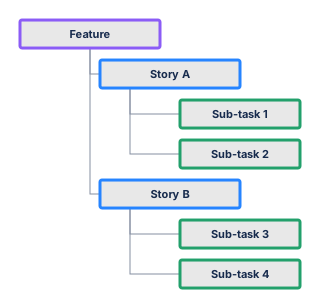
Delivery Trajectory doesn't inherently care whether those items are called Features, Stories, Tasks, or Sub-tasks.
You configure the level that represents an atomic unit of work for your organization.
If Sub-tasks are the configured work level, the four Sub-tasks are scheduled.
If Stories are the configured work level, Story A and Story B are scheduled instead. Their Sub-tasks aren't independently scheduled.
A parent is therefore excluded from scheduling when its children are the configured work items.
If an item has no children, it is naturally a leaf node and can be scheduled unless its configured hierarchy places it beneath the selected work level.
The forecast follows the level at which you actually manage delivery.
2. Measure what the team actually delivers
The historical baseline currently uses a 14-week lookback.
Only completed work contributes to the historical measurement.
The system doesn't ask how much work a team was assigned or how much capacity someone predicted. It measures what the team actually completed.
Delivery rate
The underlying calculation is time-based.
For example, if a team completed 20 Story Points over the 14-week period:
20 points ÷ 98 days = 0.204 points per day
The system isn't fundamentally measuring "points per week." The 14-week period simply provides the historical observation window.
This lets the same model work with different estimators and different team practices.
Teams are measured independently
Each team gets its own delivery rate.
That's important because an estimator such as Story Points is relative to the team using it.
A 5-point item for one team doesn't necessarily represent the same amount of work as a 5-point item for another team.
Delivery Trajectory therefore doesn't combine their points into one organization-wide velocity.
Each team is measured against its own history.
3. Use the estimator that fits your Jira
There is always one built-in estimator that needs no configuration: the time between completions. It looks at how much calendar time typically passes between one finished item and the next for that team. That's the team's raw throughput, with no dependence on how (or whether) work is estimated.
The deterministic forecast uses the average gap between completions; the Monte Carlo forecast samples from the observed gaps (more on both in sections 8 and 9). Either way, no field configuration is required: a team that estimates nothing can still be forecast from its throughput alone.
Estimator fields (optional)
If your teams do size their work, you can base an estimator on a Jira field, most commonly Story Points. The team's historical delivery rate for that field (size completed per day) then converts a card's size into an estimated duration.
When teams use different fields
A single forecast often spans multiple teams, and they don't always size work the same way: one team uses Story Points, another a T-shirt-size field, another its own custom estimate. To handle that, an estimator can list several fields in priority order:
- Story Points
- T-shirt Size
- Custom Estimate
For each card, Delivery Trajectory uses the first field in the list that has a value: Story Points if present, otherwise the T-shirt-size field, otherwise the next. That lets one estimator work cleanly across teams with different estimation practices, without forcing everyone onto the same field.
What happens when a card has no estimate?
Missing values aren't treated as zero work. If a card has no value in any of the configured fields, Delivery Trajectory substitutes the team's average size for that field across the rest of the backlog, so an unestimated card is modeled as a typical card for that team, rather than as nothing.
If there's no usable size or rate to work from at all, the item falls back to a nominal one-day duration. This keeps imperfect Jira data usable without pretending that missing information means no work.
4. Build a schedule across teams
This is where the forecast becomes more than a velocity calculation.
The forecast starts at time zero: now.
Delivery Trajectory considers the unscheduled work and determines what each team could work on next.
For each candidate item, it calculates the earliest time it could start based on:
- When the team's currently scheduled work finishes
- When its dependencies finish
- Any configured earliest-start date
- Contention with other work over a shared resource
The item with the earliest valid start is scheduled, and the process repeats until every item is placed. When two items could start at the same time, their order is broken by sprint membership first, then by Jira rank (see sections 6 and 7).
One delivery dimension per team
In reality a team has many cards in flight at once. Rather than trying to model exactly how those cards divide a team's attention, Delivery Trajectory represents each team as a single stream of throughput over time.
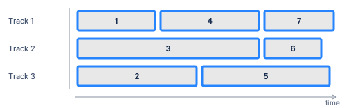

This doesn't claim the team finishes one card at a time, or that only one person can touch one card. It models how much work the team gets through over time (which is what matters for forecasting) without pretending to know exactly how attention is split moment to moment.
5. Dependencies change the schedule
Dependencies are configured using Jira issue links.
You define which relationship represents a dependency and which side is the predecessor.

The UI work cannot start until the API work is complete.
But the important part is what happens in between.
If the API is delayed, the UI team doesn't simply stop existing.
It can move to other eligible work.
When the API becomes available, the UI work becomes eligible again.
That can change what the team does next, which can change the timing of other work downstream.
Across teams

The Product team's API can't start until the Platform team's Database work is done, and the UI can't start until the API is done.
If the Database work is delayed, the Product team may temporarily work on something else. When it eventually completes, the API becomes available.
That can move the API (and the UI depending on it) earlier or later relative to the rest of the Product team's work.
Dependencies don't simply adjust dates. They can change the sequence of work.
That's why dependencies are part of the scheduling algorithm itself.
6. Other constraints
Dependencies aren't the only things that can constrain a schedule.
Earliest start date
Some work simply cannot begin before a particular date: a third-party contract that takes effect October 1, an environment that isn't available until then, and so on. There doesn't need to be a competing work item or a delivery-rate limitation; the work just can't start yet.
You can designate a Jira date field for this. When an item (or any of its ancestors or descendants) has a value in that field, the scheduler won't start the item before it, using the latest such date found across the hierarchy.
Contention
Some resources or systems cannot be used by multiple pieces of work simultaneously.
Contention is configured using a Jira field and a hierarchy level. When two items share the same value in that field, they can't be scheduled at the same time: once one holds the resource, the other has to wait until the relevant contention scope is released.
Contention can also apply above the scheduled work level. Configured at the Feature level, for example, two Stories within the same Feature collectively hold a contention value until both are complete. This keeps the forecast from interleaving work that can't actually happen concurrently.
Rank
When two items could otherwise start at the same time, Jira's Rank breaks the tie, using the same ordering you establish when you move cards up and down in Jira. (Work already committed to an active or recent sprint takes precedence first; see section 7.)
Delivery Trajectory uses that existing ordering rather than asking you to maintain another prioritization system.
7. Account for work already in progress
An active sprint contains information about work the team has already committed to.
Delivery Trajectory uses that information.
For work in an active sprint, the model can compress the item's modeled duration so that it fits within the remaining sprint.
It does not expand the team's capacity to fill the sprint.
In other words, an active sprint provides evidence about what the team is already attempting to accomplish; it isn't treated as a guarantee that the team has unlimited capacity to make everything fit.
8. Deterministic forecasting
The deterministic forecast uses the team's historical delivery behavior to produce a single projected schedule.
At a high level:
Remaining work ÷ observed delivery rate = projected delivery time
But the final result is determined by the scheduler, not just that equation.
Dependencies, contention, rank, start-date constraints, multiple teams, and the hierarchy all affect where individual work can appear on the timeline.
The result is a projected completion date for each scheduled item and the larger pieces of work that contain it.
9. Monte Carlo forecasting
A deterministic forecast gives you one projection.
Monte Carlo forecasting shows the range of outcomes that emerges when historical delivery behavior varies.
The default is 1,000 simulations, although the number can be changed for a forecast run.
Each simulation runs the same scheduling algorithm as the deterministic forecast.
The difference is how the time required for each item is determined.
Instead of returning one fixed value, the Monte Carlo estimator returns a pseudo-random value derived from the team's historical data.
The size of the work matters
Simply drawing a random historical duration for every card would ignore an important relationship: a small piece of work shouldn't share the same range of outcomes as a much larger one.
So when it samples, Delivery Trajectory weights the draw toward the historical observations closest in size to the item being forecast. A small item draws mostly from how small work has actually gone; a large item draws from how large work has gone.
The result is still driven entirely by your team's real history. The model doesn't assume delivery follows a tidy statistical curve; it uses the distribution your team's actual completions produced.
10. Dependencies run inside every simulation
This is an important distinction.
The Monte Carlo process doesn't calculate independent completion dates and then add dependencies afterward.
Each simulation runs the same scheduler used by the deterministic forecast.
The difference is that the estimated duration of each item varies.
That means:
- An item receives a simulated duration.
- Its position on the timeline is determined.
- Dependencies affect when other work can begin.
- Teams may select different work as a result.
- Those changes propagate through the schedule.
Repeat that process hundreds or thousands of times and you get a distribution of possible completion dates.
For every scheduled item, and for the larger work that rolls up from it, the simulations produce a collection of possible completion dates.
11. Read the probability curve
The Monte Carlo result is displayed as a distribution over time.
- X-axis: completion date
- Y-axis: percentage of simulations that completed on that date
The resulting curve might resemble a bell curve, but it isn't assumed to be one.
Real delivery data can produce:
- Multiple peaks
- Asymmetric distributions
- Long tails
- Other irregular shapes
The curve is simply the distribution that emerged from the simulations.
A configured commitment/end-date field can be displayed alongside the forecast, allowing you to compare the projected distribution with the date the organization has committed to.
The question becomes:
How does the current trajectory compare with the date we're committed to?
12. Roll the forecast back up the hierarchy
The schedule is built from individual work items, but the results don't stop there.
A parent's projected completion is derived from its children.
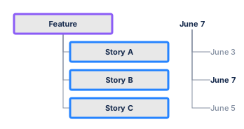
The parent's completion is the latest completion among its scheduled children. Here, Story B finishes last on June 7, so the Feature is projected to complete June 7 as well.
The same principle works through deeper hierarchies.
This means larger work doesn't need a separately maintained forecast date.
Its forecast emerges from the work underneath it.
13. What the model deliberately doesn't do
Delivery Trajectory doesn't ask you to build a detailed future capacity plan.
You don't have to manually model:
- Individual developer availability
- Vacation schedules
- Allocation percentages
- Utilization
- Planned staffing
- Expected productivity changes
These things can matter.
But attempting to predict every future change can create another model that requires constant maintenance.
Instead, Delivery Trajectory observes the team's actual delivery behavior.
If the team changes, its observed behavior can change.
If the team becomes more effective over time, that can appear in the historical data.
What it does instead, and the assumption that introduces
Instead of modeling capacity, Delivery Trajectory measures the outcome that capacity produces: how much the team has actually delivered over time. This sidesteps a hard modeling problem. Headcount doesn't convert linearly into output (the core observation of Brooks's The Mythical Man-Month: coordination cost grows with team size, so effort doesn't divide the way person-hours suggest). Rather than trying to model that, the observed delivery rate already contains it: if coordination overhead is slowing the team, or a recent hire is still ramping up, or the team has genuinely gotten faster, the rate reflects it.
The assumption this introduces is straightforward: that a team's recent delivery behavior is a reasonable basis for projecting its near-term delivery. The model doesn't assume adding 20% more people yields 20% more output; it doesn't reason about team mechanics at all. It observes the result.
14. What the forecast assumes
The fundamental assumption is simple:
Historical delivery behavior contains useful information about future delivery behavior.
That doesn't mean the future will exactly repeat the past.
It means the past is evidence.
The forecast also depends on the information represented in Jira.
If work isn't included by the selected JQL, it isn't forecast.
If a dependency isn't represented or configured, the scheduler can't account for it.
If estimation information is missing, the configured fallback behavior is used.
The forecast therefore doesn't claim to know what Jira doesn't contain.
15. The calculation stays with the data
Once Jira data has been retrieved, the forecasting calculations run in the browser.
The deterministic schedule and Monte Carlo simulations are calculated locally.
Your forecasting dataset isn't sent to a separate forecasting service to perform the calculation.
That keeps the forecasting engine self-contained and means the forecast can be calculated without sending the underlying dataset somewhere else.
Jira data retrieval is paginated so that larger datasets can be loaded incrementally.
The practical limit is ultimately the resources available on the machine running the forecast.
The pipeline in brief
Put together, the whole process is a short pipeline. It starts with your Jira data: the work hierarchy, estimates, status, teams, dependencies, rank, and any constraints. From the completed work, it measures each team's historical delivery behavior and turns that into a delivery rate.
Those rates feed the scheduling engine, which places every item on a timeline while respecting team availability, dependencies, rank, contention, and earliest-start dates. The deterministic forecast produces one projected timeline from that; the Monte Carlo forecast runs the same scheduler many times to produce a probability distribution. Either way, the output is a set of projected completion dates for individual work items and for the larger work that rolls up from them.
The model isn't trying to eliminate uncertainty. It's trying to use the information that already exists to make that uncertainty visible.
Build the best forecast the available information can support. Then make it cheap enough to redo when the information changes.